Optimization is a central component of Machine Learning, allowing models to be fit to data and thus trained. At the same time, the term and the methods that fall under it are abstract and intangible to many people.
Already in school mathematics, optimization is used to find minima and maxima (low and high points) of functions. In general, optimization problems aim at determining the combinations of certain adjustable quantities (parameters) that yield the best result with respect to a given task. Such problems occur in various domains:
- Economy: To maximize profits, the ideal determination of prices, labor distribution, personnel, etc. must be found.
- Logistics & Shipping: The positioning of distribution centers is to be evaluated so that the average required delivery time can be minimized.
- Physics: The energy minimum in a physical system is to be investigated.
- Climate research: Statistical climate models must be adapted to real measured data, which originate from complex hydrodynamic processes.
As it turns out, optimization is used in a variety of research areas and application contexts. In Machine Learning, it allows to fit a model and its parameters in training to the data at hand (like the climate example above).
How good is the model? – The objective function
In Machine Learning, parameters influence the behavior of a model. With the help of optimization, the optimal assignment of the parameters is to be found. For this purpose, training data with labels are used, for which the model can make predictions with concrete parameter assignments. From the predicted labels and the known, correct training labels, the quality of this assignment can be estimated (average error). This gives possible objective functions for optimization problems, for example: find the parameters and corresponding model prediction, with …
- … the smallest (squared) deviation (least squares)
- … the highest plausibility (likelihood)
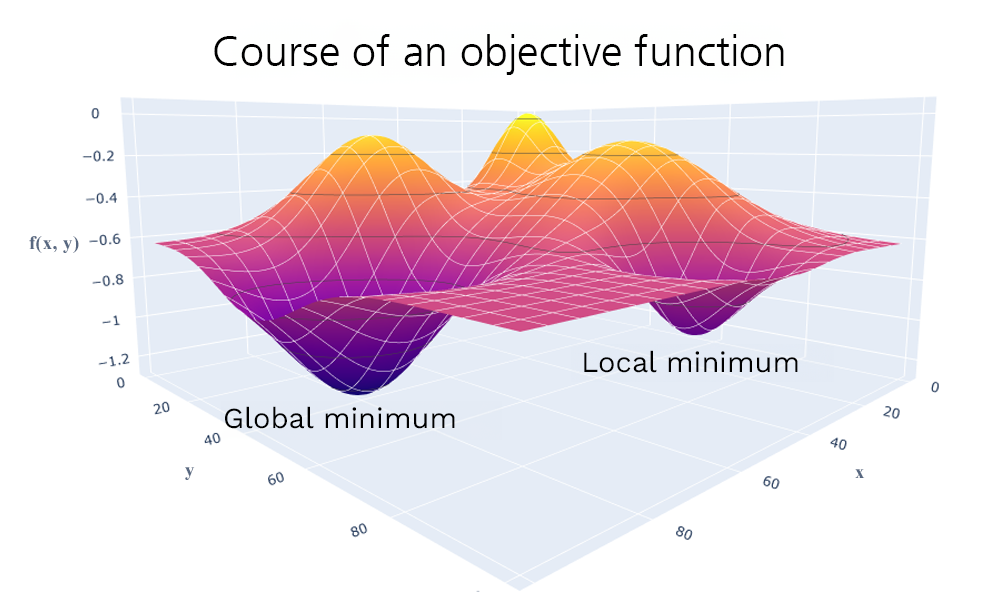
The objective function is also often referred to as loss, quality, or fitness function. Since intuitively loss should be minimized and goodness and fitness should be maximized, the corresponding objective functions are usually inverted (minima are then maxima). For a low dimensional parameter space, the function can also be represented graphically. The optimal solutions correspond here to the low points or valleys. A distinction is made between local minima, which are optimal only in a certain environment, and global minima, which have the lowest objective function value for the entire parameter space.

Two-dimensional parameter space x, y with associated objective function values f(x, y), a local minimum at x=40, y=80 and a global minimum at x=80, y=40.
Solving an optimization problem
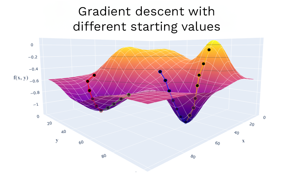
Depending on the objective function, there are different approaches to solving the optimization problem. For some functions (continuous and differentiable) optima can be determined by the derivatives of the function (necessary and sufficient criterion for first and second order gradients). However, for a large parameter space, this problem cannot be solved in a mathematically closed way. Instead, gradient descent methods can be used here, in which the optimum is approached step by step. Starting from a starting position, the gradient is alternately calculated with the current parameters, and a change of the parameters in the direction of the gradient is made until no more improvement can be achieved. For many methods (for example artificial neural networks) the current gradient is only estimated stochastically (for a part of the data). Accordingly, fewer predictions and gradient calculations are needed. This speeds up the stepwise optimization.

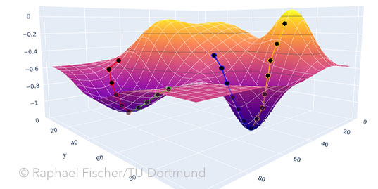
A gradient descent approaches the minimum step by step, based on the calculated or stochastically estimated gradients of the current position in the parameter space. Depending on the choice of the starting point, however, only local minima may be reached, which is why the procedure is often started and executed several times in practice (here exemplarily with four starting values).
If no gradients can be determined, one can try to search the parameter space systematically. Well-known representatives of this idea are the interval bisection method, the golden section method, and the Nelder-Mead method. They subdivide the parameter space iteratively and thus try to find lower and lower values for the objective function.
Gradient descent and search methods, however, usually find only local minima, depending on the chosen starting point. Multi-start methods can be used to perform several optimizations in parallel. Thus, several local optima can be found, among which a global optimum can also be found. Evolutionary algorithms, which are based on the theory of evolution, follow a similar idea. These procedures change step by step (generations) a group (population) of parameter assignments (individuals). By means of certain mutation and recombination methods, new assignments are generated, a part of which (depending on their usefulness) “survives” for the next generation.
Optimization as the key to the goal
Optimization is possibly the most important key component in Machine Learning, as it drives the entire learning or training process. The sub-steps of optimization sound complex at first but are usually handled fully automatically by computers. Thus, for the better-known Machine Learning methods, the associated optimization procedures are already implemented and available, they are merely configured via some set screws/hyper parameters (step size, number of starting points, etc.). However, a deeper understanding of optimization is essential to achieve good results even when the data is difficult, or the learning problem is particularly complicated. In our fourth article of the ML-Basics series, we explain which tools are relevant for Machine Learning in practice.
