When heavy rain is forecast, local authorities face decisions before they know exactly how the situation will unfold. Where should emergency teams focus their attention? Which protective measures should take priority? AI-based flood prediction can help inform these decisions, but it must provide useful information while there is still time to act.
DeepWaive is a deep learning model from FloodWaive that can reduce calculation times for flood scenarios from hours or days to seconds or minutes. Together with WestAI, FloodWaive investigated how to train the underlying models efficiently and adapt them to regional conditions. This article explains our approach and shows how DeepWaive is used in practice.
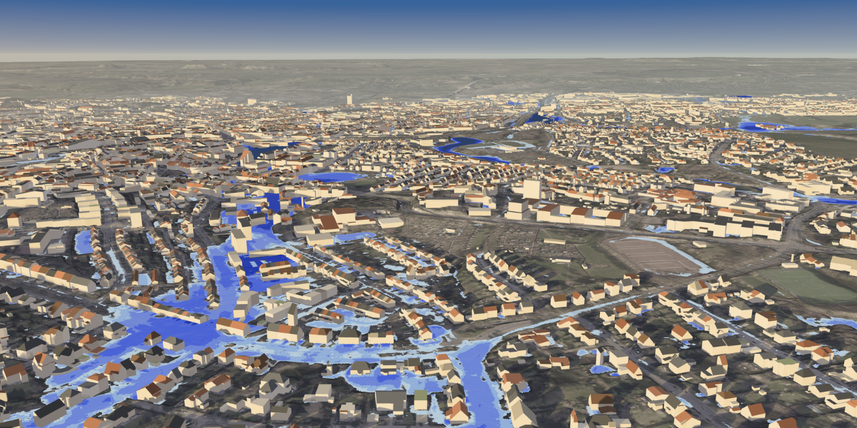
A rainfall forecast describes the weather approaching a region. Estimating its consequences requires detailed maps of how water will move through that region. They show which streets become flow paths, where water accumulates, and how water depth and flow speed change over time. These details matter to municipalities assessing which roads, buildings, and infrastructure are at risk. However, producing such flood maps for several plausible rainfall forecasts creates a substantial computational workload, often requiring hours or days of calculation.
DeepWaive learns from hydrodynamic simulations to accelerate this calculation. Its rapid predictions rely on preparation done in advance. It includes (1) generating reference scenarios, (2) training the AI model on these scenarios and (3) testing how well the model performs on new, unseen situations. Our research cooperation with WestAI examined how to make that preparation more effective. We investigated the resources needed for a reusable base model and the extent to which local adaptation could improve regional performance without repeating the full training process.
From rainfall to flooding
Hydrodynamic modelling shows how terrain, rainfall and other event conditions shape the movement of water. A digital elevation model describes the height of the ground surface as a detailed map, while buildings and other obstacles influence possible flow paths. Rainfall, water flowing into the area from outside and the water already present determine how the simulation develops.
In a typical numerical approach, the surface is divided into computational cells. Physical equations describe how water moves between neighbouring cells and how the flow changes over successive time steps. The resulting maps show water depth above the ground and flow velocity, including its direction. Because the cells interact, conditions upstream can affect flooding some distance away. For example, representing a building as impermeable redirects the calculated flow through neighbouring cells.
The simulation depends on its input data. For an operational forecast, rainfall may come from a weather prediction. For a training scenario, it can be deliberately specified. Consequently, several weather forecasts can produce different flood maps for the same terrain. This keeps the uncertainty about the approaching weather separate from the calculation of its possible effects on the ground.
Finer spatial resolution increases the number of interacting cells, while longer events require more time steps. Repeating the simulation for alternative rainfall patterns adds further runs. This is valuable for exploring possible outcomes. However, the high computational demand limits how many scenarios can be assessed in the short time available before a warning has to be issued.
Learning a reusable flood surrogate
DeepWaive is a learned approximation, or surrogate, of this numerical calculation. In simple terms, it learns to predict flood maps without running the full simulation every time. For training, terrain and event inputs are paired with flood maps generated by hydrodynamic models. The network compares its predictions with those references and adjusts its parameters to reduce the difference. Its transformer architecture allows the model to represent relationships between different locations in the input. This is important when the evolution of flooding at one location depends on conditions elsewhere.
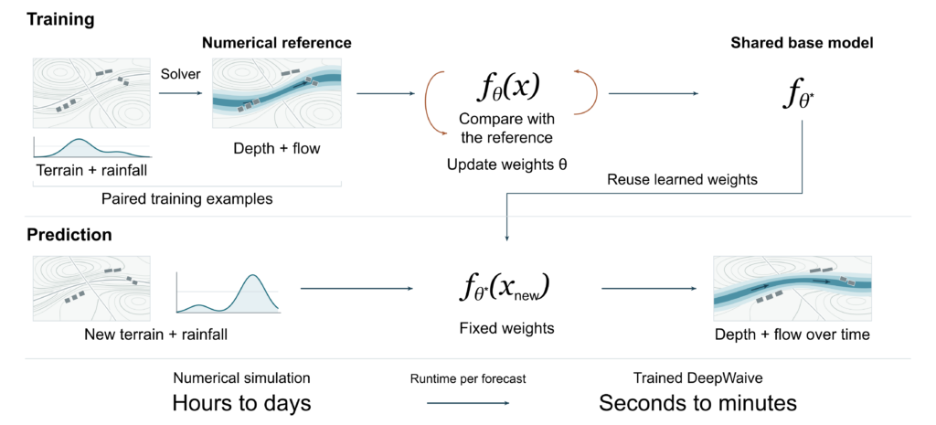
Figure 1. Numerical simulations provide the reference maps for training DeepWaive. Once trained, the model’s learned parameters (weights θ*) are reused for new forecasts. Prediction can take seconds to minutes instead of the hours to days needed by a numerical solver. Actual runtimes depend on the area, resolution, event duration and hardware. © FloodWaive.
Simulation makes it possible to construct varied training scenarios, including events for which detailed observations are unavailable. Each simulation links prescribed input conditions such as rainfall and terrain to the corresponding flood dynamics. This provides one route to incorporating physical knowledge into machine learning.
Generating reference scenarios and training the network are compute-intensive preparation steps that are completed before operational use. The time savings then apply to every prediction. Once trained, DeepWaive processes new terrain and rainfall inputs with fixed weights, without rerunning the full numerical simulation or fitting the model for each forecast. Figure 1 shows these stages.
We describe this reusable network as a foundation model for flood prediction. It is a common base model trained on many different scenarios and intended for use across multiple regions. For a new region, the model receives that region’s terrain map as input. Adapting the model goes a step further and changes what it has learned. Local reference simulations can support this adaptation where predictions need to match local conditions more closely. This creates two related investment decisions: how much to learn through broad training, and how much to adjust for a particular application.
Matching model capacity to the workload
The cooperation brought together three elements: FloodWaive’s DeepWaive model and simulation pipeline, research on adaptation methods at the Laboratory for Machine Tools and Production Engineering (WZL) of RWTH Aachen University, and WestAI computing resources on the university’s high-performance computing cluster CLAIX.
Our starting point was the approach established in scaling studies of language models. These studies examine how prediction quality changes when model size, training data and computing power are increased. Additional parameters can represent more complex relationships, but their benefit depends on having enough training examples and computing effort to make use of them.
We compared three model sizes of roughly 125 million, 500 million and 2 billion parameters. For the training setup examined, the comparisons identified around 500 million parameters as the best balance between prediction quality and training effort. Frequent forecasts shift the emphasis to inference cost, which is the time and computing power needed to run the model for each prediction. For this reason, FloodWaive continued developing larger and more compact variants suited to different workloads.
The allocation of graphics processing units, or GPUs, presented a separate engineering trade-off. Training on several GPUs in parallel splits up the computation, but the GPUs must exchange information to keep their copies of the model in sync. In our tests, around eight GPUs gave the best ratio of prediction quality to resource use. We attribute the limited benefit of using even more GPUs mainly to communication overhead, meaning delays caused by data exchange between GPUs.
Data volume and coverage answer different questions
Our tests suggest that the benefit of additional training data depends on how varied the scenarios are and on how much data the model has already seen. To our surprise, the gains in prediction quality levelled off in some experiments when more examples of a similar kind were added. We interpret this as a sign that the tested model had learned most of what it could from this type of data.
A separate FloodWaive development test in September 2025 identified a more specific gap in scenario coverage. In this test, water was allowed to accumulate behind a barrier in a simulated landscape. The calculation was then continued from that point with the barrier removed. In the model’s prediction, the accumulated water remained in place instead of flowing away. This transition, in which a barrier disappears while water is held behind it, had not been represented in its training scenarios.
The test suggested a targeted extension to the training set to address this gap: scenarios in which barriers appear or disappear during an event. After training, the resulting flow response should be carefully evaluated. Further examples with unchanged obstacles would not directly supply that missing transition. Figure 2 illustrates the model response observed in the development test and the physical behaviour that motivated the proposed additional training.
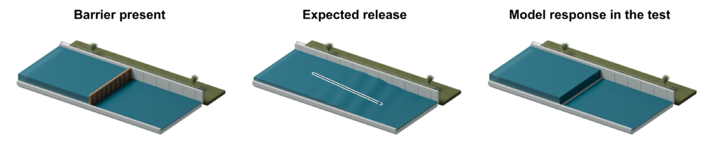
Figure 2. This schematic shows a FloodWaive development test that started from a state where water had accumulated behind a barrier. The barrier was then removed. The two right panels compare the expected release (water flowing freely) with the model response in the test (water remaining trapped). This finding suggests adding training examples that include changing obstacles, such as barriers that appear or disappear during a flood. © FloodWaive.
Adapting the shared model to regional conditions
Local adaptation provides another use for additional examples. Regional reference simulations may differ from the broad training corpus (the large, diverse dataset used for initial training). These differences can include how the terrain is represented and which modelling assumptions are used. This makes regional simulations valuable for adapting the base model to a particular area. We evaluated regional adaptation using reference simulations for StädteRegion Aachen, the regional district that includes the city of Aachen.
Full fine-tuning trains the whole base model further on regional data, and all of its parameters can change. This approach builds on what the base model has already learned and gives it full flexibility to adapt to the region. The trade-off is that a large network has to be optimised and each region gets a complete model of its own that must be maintained separately. We compared this approach with alternative methods that restrict which parameters are adjusted during adaptation.
With low-rank adaptation, or LoRA, the pretrained weights remain fixed. Instead of changing all parameters, the model learns a small correction for regional adaptation. This correction is represented by the product of two smaller matrices. Restricting their rank limits how flexible the correction can be. This substantially reduces the number of trainable parameters compared with full fine-tuning. The prediction combines the original transformation with this learned correction. Figure 3 shows the relationship between the frozen weights and the trainable components.
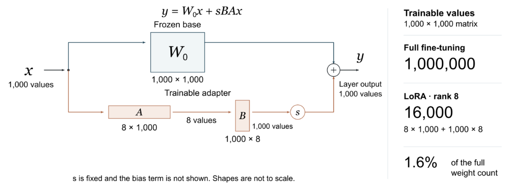
Figure 3. LoRA combines a frozen transformation W₀ (the original, unchanged model weights) with a trainable correction sBA. For a 1,000 × 1,000 layer with rank 8, the adapter contains 16,000 trainable values, just 1.6% of the original weight count. Regional adaptation changes only A and B. The scaling factor s is fixed, and the bias term is not shown. © FloodWaive.
We also investigated weight-decomposed low-rank adaptation, or DoRA, a related method. DoRA splits the model’s pretrained weights into two components: magnitude (size) and direction. It updates the magnitude separately and applies low-rank adaptation to the direction. Integrating these methods required work on the existing model architecture, so we developed our own LoRA and DoRA components. An early prototype had shown that standard adapter software could not be applied directly to the model’s attention layers. We reviewed the mathematics of our components, especially where the adapters were placed and which parameters were allowed to change during adaptation.
In the collaboration’s comparisons, LoRA and DoRA approached full fine-tuning performance. At the same time, they needed far fewer trainable parameters. Their modular structure also simplifies deployment. Regional adapters can be stored separately and combined with a shared base, which reduces duplication across regional models.
Evaluating transfer and local improvement
The intended use of a model determines which data must be held back from training for its evaluation. A foundation model should also work in regions it has never seen. This transfer is tested on geographic areas that were excluded from base-model training. Regional adaptation raises a different question: does the adapted model improve predictions for events over the same terrain that were not used for fine-tuning? Figure 4 distinguishes these forms of generalisation, meaning the model’s ability to perform well on new, unseen data.
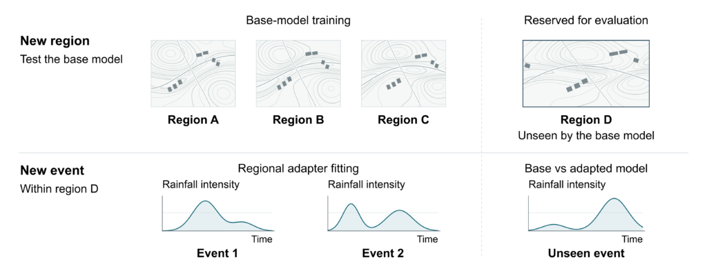
Figure 4. Generalisation should be tested for both new regions and new events. In the diagram, region D is excluded from base training. Adaptation uses selected local events, with a separate event reserved for comparing the base and adapted models. © FloodWaive.
Spatial evaluation must also consider the features that matter for real-world decision-making. For example, close agreement across much of a map can coexist with a critical error in a predicted flow path. Such an error could lead authorities to misjudge whether a road or building is at risk. Therefore, examining the extent of flooding, changing water depths and flow patterns helps interpret an overall accuracy score. Water balance adds a physical consistency check by relating water entering, leaving and remaining within the area.
Connecting efficient training to operational forecasting
Since May 2025, StädteRegion Aachen has been using the AI-supported flood early-warning system developed with FloodWaive. The system calculates its flood maps with DeepWaive. In such an operational setting, total runtime includes preparing input data, running the model itself (inference), and producing usable flood maps. Accelerating the calculation leaves time to examine several plausible rainfall scenarios. It also means the predicted consequences can be updated whenever the forecast changes.
Our work with WestAI looked at which development choices serve that goal. For the configurations examined, the training comparisons found the best balance at around 500 million parameters. The data experiments and the separate barrier test indicated that the range of situations covered by the training data matters as well as its amount. In the adaptation experiments, LoRA and DoRA adapters came close to full fine-tuning with far fewer trainable parameters. Future development therefore focuses on identifying the situations that call for additional training scenarios and on testing whether the resulting improvements carry over to unfamiliar events.
Acknowledgements
The research cooperation used computing resources granted by WestAI.