Two Pruning Algorithms: MEP vs. PEP – one Goal, different Outcomes

Recap: What is Decision Tree Pruning?

Decision trees provide a practical and straightforward way to represent rules based on existing knowledge or decision processes for classification. However, they tend to overfit and can become very complex and large as the amount of data grows. Using pruning algorithms is a solution to address this problem. These algorithms remove redundant and unimportant differentiations, cutting specific branches in the tree to make it smaller and more manageable. We have described exactly how this works in our last blog post. Various pruning algorithms differ in terms of the direction in which the tree is traversed or their pruning criteria, which determine when a branch should be pruned. In the following, we will take a closer look and compare two of such algorithms.

Pessimistic Error Pruning (PEP)

The Pessimistic Error Pruning algorithm is a top-down pruning algorithm. This means we start at the root and then, for each decision node, we check from top to bottom to determine whether it is relevant for the final result or should be pruned. For each node t, we calculate the following:

• The error of the node, e(t), errechnen wir als Summe der falsch zugeordneten Samples (d.h. Samples, die nicht der Mehrheitsklasse zugeordnet wurden) addiert mit einer Kontinuitätskorrektur von 1/2 im Fall von binären Entscheidungen. Dies machen wir, um einem Bias entgegenzuwirken, der entstehen kann, wenn das gleiche Set von Samples sowohl für das Erstellen als auch das Prunen eines Baums verwendet wird.
• The error of the subtree of the node, e(T_t), is calculated as the sum of the errors of all the leaves following node t (including continuity corrections).
• The standard error is now calculated from these two results and n(t), which describes the number of samples in node t:

Pruning occurs when the sum of the standard error and the error of the subtree is greater than or equal to the error of the node. This happens because node t, as a leaf node, makes fewer errors than the subtree.

This is illustrated in the following example:

We consider a database containing various types of Iris flowers and classify them based on their different petal and sepal sizes. The 150 flowers can be sorted into three subtypes (setosa, virginica, versicolor). Initially, we classified these using a decision tree based on attributes. In the following, we apply both pruning algorithms to this tree and explain what happens during pruning in each case.

For the Pessimistic Error Pruning Algorithm (PEP), let’s examine three nodes in the depicted tree as an example. We start with Node A, which is the root node. Since the algorithm is a top-down algorithm, the root is the first node considered by the algorithm. Here, 79 samples were not assigned to the majority class (marked in blue), resulting in an error of 79.5 (including the continuity correction) for the root node. The error of the subtree at the root node is 4 since there are a total of 8 leaf nodes reachable from it, each with an error of 0, and the standard error is approximately 1.97 when considering the total of 120 samples in the root node. Since the error of the root node (79.5) is greater than the sum of the subtree error and standard error (4 + 1.97 = 5.97), the pruning criterion is not met, and pruning does not occur.

Now, let’s look at the two nodes in the tree that meet the pruning criterion: Leaf Node B has misclassified 1 out of 37 samples, resulting in a node error of 1.5. There are 3 reachable leaf nodes, each with an error of 0, resulting in a subtree error of 1.5 and a standard error of approximately 1.19. Thus, the pruning criterion is met because the node error is less than the sum of the subtree error and standard error (1.5 < 1.5 + 1.19). For Node C, this is also the case with 1.5 < 1 + 0.99. Therefore, pruning occurs for these nodes, and the underlying subtrees are cut. The nodes are transformed into leaf nodes. This process not only makes the tree more compact but also improves accuracy, increasing it from 93% to approximately 97%.

Minimum Error Pruning (MEP)

The other algorithm we are considering traverses the tree in a different manner (bottom-up). The tree is traversed from bottom to top, moving from the leaves to the root. Additionally, a different formula is used to evaluate our nodes.
The basic principle here is that we compare the error of a parent node with its child nodes. This allows us to determine whether the child nodes will improve the error or not. If the subordinate nodes have a lower error, they positively contribute to the result and are retained. However, if the error of these nodes is higher, their presence worsens the result, and as a result, they are removed.
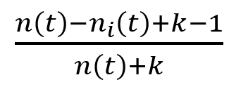
To calculate the error of the parent node, we use a parameter, denoted as m, which originally determines the influence of the a priori probability p_ai that a sample does not belong to a specific class:

For simplicity, we can set to 1/number of classes(k) and m to the number of classes, effectively removing the a priori probability “p_ai” from our error calculation formula: 

To compare this error with that of the child nodes , we need to aggregate the errors of them. It is important that the node that makes decisions based on more samples is evaluated with a higher weighting. These weights determine the influence of each child node as they describe the probability of a sample going to the respective child node. As mentioned earlier, now the error of the child nodes must be greater than that of the parent node in order for us to prune the subtree.
This principle is now demonstrated on the same tree as the first algorithm:

Since MEP is a bottom-up algorithm, we first look at the leaf nodes labelled A and B in the figure. To decide whether they should remain part of the tree or be pruned, we need to compare their shared weighted error with that of the parent node. Both childnodes have the same weight and the same error since each has one sample correctly classified in the respective node. In this case, the shared error is 1/2. The error of the parent node of these child nodes (Node C) is 3/5. Therefore, the error is minimized in the case of the child nodes A and B, so they remain in the tree.

In the next step, we move one node higher and compare nodes D and C with their parent node E. Both D and C have an error of 0.082, and E has an error of 0.075. In this case, it is the other way around. The child nodes of node E worsen the error, making them unusable for our decision tree. Therefore, they are pruned, reducing the size of the decision tree.

The remaining comparisons in the tree do not lead to further pruning, and our decision tree is complete.

Comparison of the two algorithms

Both algorithms share the same fundamental principle, which is the evaluation of the importance of nodes. The biggest difference lies in the direction of processing. In general, top-down methods are considered riskier because they may cut important branches uncontrollably. PEP ensures, through the pruning criterion, that pruning occurs in the right situations and with sufficient frequency. On the other hand, the Minimum Error Algorithm is very cautious and prunes relatively infrequently, resulting in few notable improvements. Therefore, in most cases, the MEP algorithm is the less favorable choice, even though it is the less risky principle.

This is illustrated in the following example:

This dataset pertains to the classification of breast cancer, where attributes like tumor size or concavity are used for categorizing tumors as benign or malignant. Both algorithms can shorten decision trees for this dataset. When PEP was applied to a decision tree in this dataset, the number of leaves was reduced from 19 to 8, clearly indicating that the tree became more manageable. Additionally, the error rate decreased as two more samples were correctly classified from the data used to test the tree. MEP pruned the tree used in the dataset from 15 leaves to 13, with no improvement in the error rate. Consequently, we find that PEP delivers better results even for this dataset.

Conclusion

In conclusion, it is evident that the choice of algorithms can be very relevant, even though both aim to achieve the same goal. Minor differences in algorithms can impact the result, which, in the case of the Pessimistic Error Pruning Algorithm, is definitively better. However, it is important to note that these algorithms are not the only pruning algorithms available, and different algorithms may be suitable for different trees/applications. In summary, it is worthwhile to consider which algorithm to use for a specific problem.

Datasets used:

Both the Iris dataset and the breast cancer dataset, which we used to create the decision trees, are from scikit-learn:

Iris flowers: https://scikit-learn.org/stable/auto_examples/datasets/plot_iris_dataset.html

Breast cancer: https://scikit-learn.org/stable/modules/generated/sklearn.datasets.load_breast_cancer.html