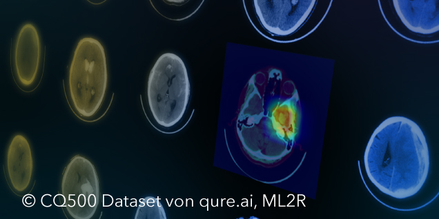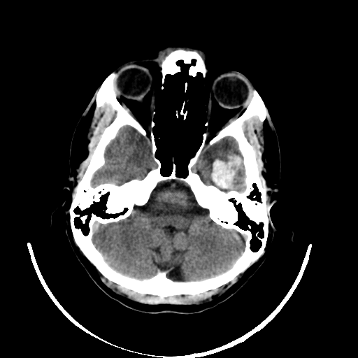
“Time is brain” – this well-known phrase encapsulates the challenge of a stroke. When a person suffers a stroke, quick action is crucial to minimize lasting damage. The cause of a stroke can be either a vessel blockage (ischemic) or bleeding in the brain (hemorrhagic). While blood-thinning medications can restore blood flow in the case of a vessel blockage, they would be counterproductive in the event of bleeding. Therefore, imaging diagnostics are essential to quickly differentiate between these two conditions and, in the case of a hemorrhagic stroke, examine the location and size of the bleeding. Typically, a Computed Tomography (CT) (see Figure 1) scan of the skull is performed, consisting of multiple individual images (layers) that collectively create a three-dimensional impression of the head.

Figure 1: CT scans of the skull showing bleeding in different regions of the head.
The analysis of CT scans can be time-consuming and challenging, especially for early-career medical professionals. To address this issue, the idea emerged to support physicians through an application that automatically classifies whether bleeding is present in a computed tomography. The use of Deep Learning, particularly Convolutional Neural Networks (CNNs), is well-suited for this task. In safety-critical fields like medicine, it is imperative to ensure that physicians can comprehend the predictions of such a system.
Where do the data come from, and how does the model work?
The foundation for implementing such an application requires data. In 2018, the Radiological Society of North America (RSNA) released a dataset of CT scans as part of the “RSNA Intracranial Hemorrhage Detection” competition on Kaggle. This dataset is the largest multinational and multi-institutional collection, containing over 25,312 CTs comprising a total of 874,035 images. Radiologists labeled these images with six different classes. The first class indicates whether a stroke is present, while the other classes specify the region of the head where bleeding occurs (see Figure 1).
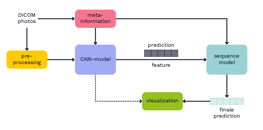
In addition to the dataset, the winning algorithm from this competition is used as the basis for the model to classify hemorrhagic strokes. Further details about the model can be found in Wang et al.’s paper, which was not yet published at the time of this work. The published model from the competition is retrained by splitting the original training dataset into new training and test datasets. The basic structure of the model is depicted in Figure 2. Initially, from the medical data in DICOM format, both image data and metadata are extracted. Metadata includes information such as the anonymous patient ID. Next, the image data undergoes preprocessing. The preprocessed images and metadata serve as input for a CNN model. The CNN model processes all layers of the CT independently, generating output for each layer indicating the presence of bleeding and its region in the brain. This output and the learned features of the CNN model are input for a sequential model. In the sequential model, the entire CT is considered a sequence. The idea is to leverage neighborhood information, such as when the same bleeding class is detected on consecutive CT layers, to improve the model. The sequential model also allows the merging of predictions and features from different trained CNN models. The output of the sequential model is again a classification for each layer of the CT.

Figure 2: Overview of the model structure.
The model is retrained using various preprocessing methods, CNN architectures, and combinations. The model embedding is adjusted so that it can process any CT as input data. Through experiments, the best model emerges as a combination of two different CNN models, whose outputs are merged in the sequential model. Both CNN models use an SE-ResNeXt-101 architecture as their backbone. This architecture combines a ResNeXt-101 architecture with a Squeeze-and-Excitation block (SE-Block), where more important feature maps are weighted more strongly. In the first model, medical input images are generated in three different windows. All three highlight different structures such as bones or soft tissues, by selecting a specific interval from the digital values of the CT scan, which are represented in the so-called Hounsfield scale. The Hounsfield scale represents X-ray attenuation in tissues. In the second model, three consecutive layers of a CT are used as input for the CNN model.
After training, the model is evaluated on two additional datasets. The first dataset is the publicly available CQ500 dataset. Here, the model produces results similar to the RSNA test dataset. Across most classes, performance metrics such as Accuracy and AUC are high (CQ500 dataset: Accuracy: 97-99%, AUC: 98-99%). The F1-score is high for almost all classes (71%-98%), except for epidural bleeding (25%). The same is observed on the RSNA test dataset, where the model seems to perform poorly due to far fewer data for bleeding in this region. Many epidural bleedings are wrongly identified as subdural. Subdural and epidural bleedings occur close to each other on opposite sides of the outer layer of the brain.
The second test dataset uses data from a local hospital. To specifically examine data from routine clinical practice, all intracranial CT images were collected over two months. Both the newly trained model and a radiologist from the local hospital classify all CT images. Subsequently, both results are jointly analyzed with the radiologist.
How can physicians understand the model’s decisions?
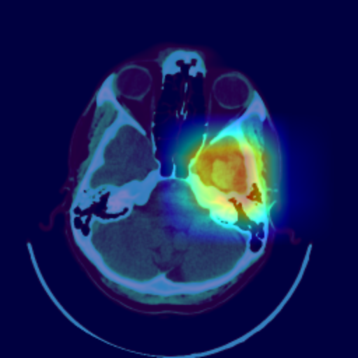
Even though the model delivers excellent results, it is crucial for discussions with radiologists and real-world application contexts to address how physicians can comprehend the model’s decision. Various post-hoc methods can explain an algorithm’s decisions retroactively. In this work, the Grad-CAM++ procedure is used. This method produces a class-specific visualization (see Figure 3), illustrating the importance of a specific region for the algorithm’s decision. The visualization is a weighted linear combination of positive gradients of the feature maps of the last convolutional layers.


The visualization allows the radiologist to understand which regions were noticeable to the algorithm and to verify the classification. In the joint analysis of the second dataset, the radiologist can confirm some spots detected by the algorithm as bleeding that were overlooked in advance. Simultaneously, the visualization shows that the model incorrectly classified several surgical defects as bleeding.
Conclusion
Deep learning often yields excellent results in the classification of medical image data. The automatic classification of hemorrhagic strokes can be realized through CNNs in conjunction with a sequential model, providing high performance in most cases. For deployment in a safety-critical area like medicine, explanatory capabilities are crucial alongside consistently high performance. Visualization through Grad-CAM++ offers a means to make the results comprehensible for physicians. It appears sensible to assist medical professionals through such an application, enabling the rapid detection of anomalies through the quick classification of CT images. Nevertheless, medical personnel should critically examine and confirm the results in each case to eliminate false predictions.
