In another blog post of this series, we introduced linear regression. We saw that by using the least squares method, we can fit a regression line to training data to predict a target function value for new, unknown data points. This allowed us to find a line in our application example that intuitively made sense:

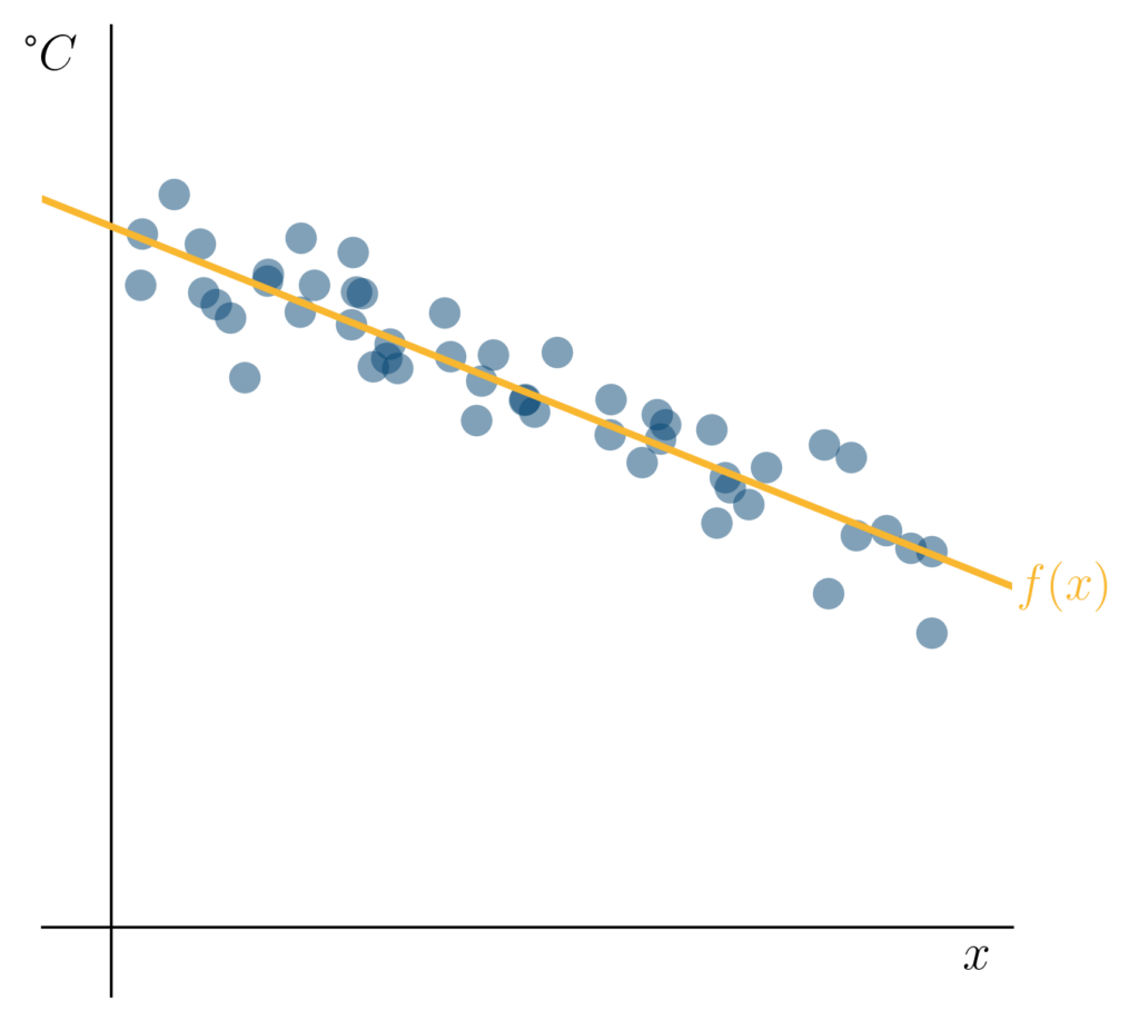
We have plotted the temperature controller settings of a refrigerator on the $x$-axis and the measured temperatures on the $y$-axis.
Let’s assume our data comes from an experiment where we measured the temperature inside a refrigerator for different settings on the temperature regulator. In this case, it seems reasonable that there is a linear relationship (the higher the regulator setting, the colder the refrigerator). It is understandable that multiple independent temperature measurements at the same setting do not yield exactly the same result. These slight fluctuations are normal and are referred to as noise. Our example above nicely illustrates this noise.
Outliers and Problems in Training
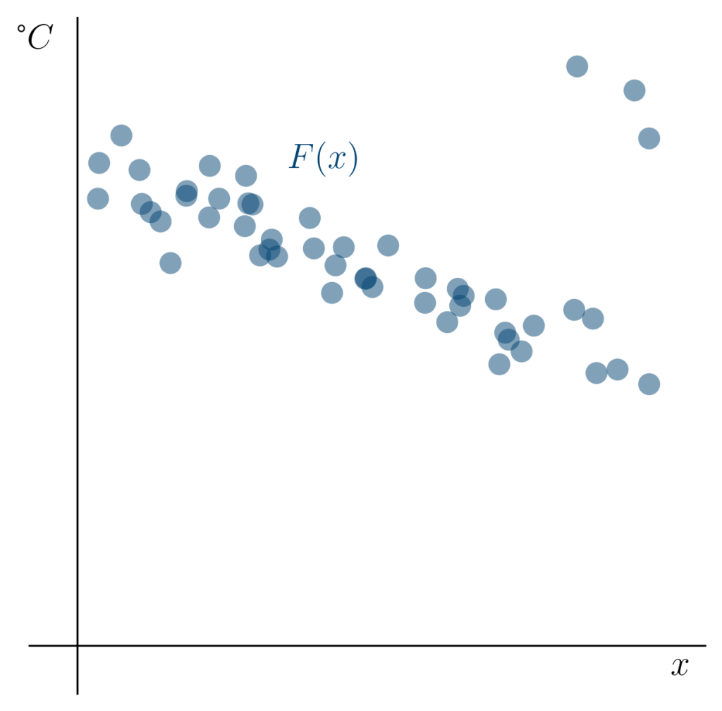
However, sometimes some measurements fail. In the following image, we have taken three additional measurements. We see three points at the upper right edge of the graph that do not follow the trend of the other measurements. Such data points are called outliers. Outliers in our refrigerator example could occur if, for instance, the thermometer malfunctions or a measurement is not conducted properly (e.g., if the door remains open for too long).

Something has obviously gone wrong here.
We would like our learning algorithm to identify the global trend of the data despite the presence of such outliers. However, if we use the least squares method for training on this data to determine a regression line $f_{LSQ}(x)$, we obtain the following result:

The least squares method reacts sensitively to our three outliers.
Our regression line $f_{LSQ}(x)$ appears to be “pulled” toward the three outliers. We can suspect that our temperature predictions for high regulator settings may no longer be accurate. Now, we will explore why this behavior occurs and how we can (partially) correct it.
Robust Linear Regression with Least Absolute Deviation
In the previous blog post, we saw that the least squares method minimizes the following error function:
$$ E_{LSQ}(a, b) = \sum_{\substack{x \text{ in amount of training}}} \left( a \cdot x + b\; – F(x) \right)^2 $$
The distance $ a \cdot x + b \; – \; F(x) $ of our training points $x$ from the regression line, described by the parameters $a$ and $b$, is squared in the error function. This means that the “cost” we pay for training points that are far from our regression line is very high. The cost increases not just linearly, but quadratically. As a result, it is often beneficial to slightly increase the small distances of many points from our line to reduce the large distances of a few points.
There are many different ways to make our regression line more robust to the data. One such method uses the least absolute deviations method, which minimizes the following error function:
$$ E_{LAD}(a, b) = \sum_{\substack{x \text{ in amount of training}}} \left| a \cdot x + b \; – \; F(x) \right| $$
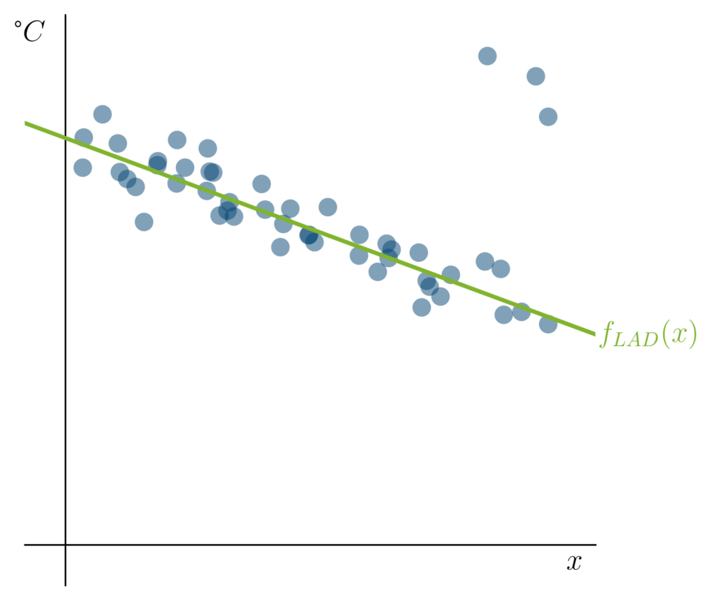
Instead of considering the squared distance to the line, this error function considers the “normal” (Euclidean) distance. When we use a method that minimizes this error function, we obtain the following regression line $ f_{LAD}(x) $ on our training data:

By modifying our error function, we have achieved that the line $ f_{LAD}(x) $, which minimizes this error function, once again aligns with our expectations. Interestingly, the idea of fitting linear models to data using the least absolute deviations method is quite old: It dates back at least to Boscovich (1757) and Laplace (1793). This means it was known even before the better-known least squares method, described by Gauss (1801) and Legendre (1805).
Why do we usually use the least squares method if it fails in the presence of outliers? The answer is that optimizing $E_{LAD}$ is more computationally demanding than optimizing $E_{LSQ}$. This is because only iterative methods are known for minimizing $E_{LAD}$, which generally require many computation steps to find an optimal solution. In contrast, an explicit formula exists for the optimal solution of $E_{LSQ}$. Nevertheless, we will now demonstrate how to practically implement an outlier-robust regression method using Python and the NumPy and SciPy packages.
Practical Implementation of Robust Linear Regression
We assume we have a Python environment with NumPy and SciPy installed, such as a locally running Jupyter Notebook or a notebook on google colab. We begin by importing NumPy, SciPy, and loading our data from a text file:
import numpy as np
import scipy as sp

data = np.loadtxt('data-outlier.csv', delimiter=', ')

vecX = data[0]
vecY = data[1]
The optimization of $E_{LAD}$ can be implemented using linear optimization. The core idea is to define a system of (linear) inequalities that specify the conditions our two regression parameters $a$ and $b$ must satisfy and to find the parameters that minimize a (linear) objective function. Fortunately, our error function $E_{LAD}$ can be represented in the necessary way. The background on these transformations is discussed in two posts in our Coding Nuggets series.
matF = np.vstack((np.ones_like(vecX), vecX))

matA = np.zeros((2*n, m+n))
matA[:n,:m] = +matF.T
matA[n:,:m] = -matF.T
matA[:n,m:] = -np.eye(n)
matA[n:,m:] = -np.eye(n)

vecB = np.zeros(2*n)
vecB[:n] = +vecY
vecB[n:] = -vecY
vecC = np.hstack((np.zeros(m), np.ones(n)))
The variables m and n represent the dimensionality and the number of data points in our dataset, respectively. We now seek the vector vecW that minimizes the expression vecW.T @ vecC under the condition that the vector matA @ vecW is never greater than the vector vecB row-wise. Here, @ represents standard matrix-vector multiplication. A method to identify such a vector vecW is already implemented in scipy.optimize package and can be called as follows:
result = sp.optimize.linprog(vecC, A_ub=matA, b_ub=vecB, bounds=(None,None))The result object contains our desired output along with additional information that we will not examine in detail here. We can now extract our regression parameters as follows:
vecW = result.x[:m]
print ('a =',vecW[0])
print ('b =',vecW[1])
This yields the parameters:
$$ a = -0.371 \quad b = 9.976 $$
The corresponding regression line $ f_{LAD}(x) $ is shown in green.
Outlook and further details
In this post, we explored how to determine a regression line using the least absolute deviations method. This method provides greater robustness against outliers in the data. We saw that our modified error function $E_{LAD}$ can be solved using linear optimization and demonstrated how this can be practically implemented in Python. In our Coding Nuggets series, we discuss the technical details of robust linear regression in more depth. Another article covers the basics of linear optimization in Python. Robust regression is highly relevant in practical Machine Learning applications and is frequently used in the context of signal processing, computer vision, and knowledge discovery.
