The currently dominant method for training Machine Learning (ML) models is gradient descent. The backpropagation algorithm, for example, made it possible to efficiently train millions of parameters in deep neural networks. This was crucial for the recent resurgence of this model class. In this process, gradients—also known as derivatives in school mathematics—of the loss function for all neurons are computed sequentially through the layers of the network, starting from the last layer. This conceptually simple method is relatively easy to implement and relies only on fundamental mathematical operations. Today, the term “training” in the context of Machine Learning is almost synonymous with gradient descent. However, there are alternative methods for optimizing models, including evolutionary optimization, which offers advantages over gradient-based methods.
Training ML models is essentially an optimization problem (Optimization in Machine Learning): Given is a dataset $\mathcal{D}$, for example, with pairs $(x,y)$ of inputs $x$ and expected outputs $y$. If $y$ is continuous, such as a real number, the problem is referred to as regression. If $y$ is instead a symbolic value from a finite set, such as “cat” from the set ${\text{dog}, \text{cat}, \text{horse}}$, the problem is called classification. A model $\mathcal{M}$ with parameters $\theta$ is capable of mapping inputs $x$ to outputs $y$, represented as
$$\mathcal{M}_{\theta}(x) = \hat{y}$$
Here, $\hat{y}$ denotes the prediction of the model, as opposed to the true value $y$, which is given by the data set. During training, we now search for the optimal parameter
$$\theta^*$$
which ensures that the model output for all $x$ from $\mathcal{D}$ is as close as possible to the true output $y$:
$$\sum_{(x,y) \in \mathcal{D}} d(y,\mathcal{M}_{\theta^*}(x))~\rightarrow ~\min$$
Here $d(\cdot,\cdot)$ is an arbitrary distance measure, in the case of a regression for example $$d(y,\hat{y}) = (y-\hat{y})^2.$$ The sum in the above example is also referred to as the loss function $L$.
Gradient methods attempt to minimize this function by taking the derivative $$\mathrm{d}L/\mathrm{d}\theta$$. Calculating the derivative is often computationally expensive. In addition, $L$ can have many different local optima or even not be derivable at all. In this case, gradient methods can either not be used effectively or not at all. The remedy in this case is evolutionary optimization.
Optimization Through Local Search
Let us take an even more general formulation of an optimization problem as a basis: From a set $\mathcal{X}$ of possible solution candidates, an element
$$x^* \in \mathcal{X}$$
is to be found which, with respect to a fixed loss function $$L:~\mathcal{X} \rightarrow \mathbb{R}$$ is minimal:
$$x^* = \underset{x \in \mathcal{X}}{\arg\min} L(x).$$
In principle, the optimal element $x^*$ could be found by drawing random elements from $\mathcal{X}$. Although this random search approach is easy to implement, it is ineffective if the search space $\mathcal{X}$ is very large. Nevertheless, it is a good reference against which other methods can be compared: If an optimization method delivers worse results than Random Search, it is not suitable for the problem at hand. In contrast to the gradient method, which starts from a starting point $$x^t$$ and moves in the opposite direction of the gradient,
$$-\eta \cdot \mathrm{d}L/\mathrm{d}x^t,$$
with step size $\eta$ in order to approach an optimum as directly as possible, _Random Search_ jumps around randomly in the solution space and tests out random solution candidates.
A middle way consists of starting from a starting point $x^0$ and feeling one’s way around this point. For example, various nearby points $\tilde{x}^0_1, \dots, \tilde{x}^0_{\lambda}$ are evaluated. The point with the lowest loss value, which therefore appears to be closer to the optimum and is therefore the most promising, is then adopted as the new starting point $x^1$. If none of the nearby solutions is better than the starting point, $x^1 = x^0$ is left as it is. If this process is repeated frequently, the point $x^t$ moves towards an optimum for an ever-increasing $t$. This scheme forms an optimization method called (1+λ)-EA. EA stands for Evolutionary Algorithm.
Evolutionary Algorithms
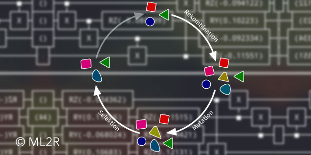
Evolutionary algorithms are a class of optimization methods that have been researched since the 1950s. The model here is evolution in nature, first formulated by Charles Darwin: when living beings reproduce, genes from the parents are recombined. In addition, mutations occur, as a result of which the offspring inherit characteristics of the parents and can spontaneously develop new characteristics. Better-adapted offspring survive and manage to produce offspring themselves. Poorly adapted individuals, on the other hand, die as a result of selection pressure, for example due to predators or limited food supply. This process is imitated in evolutionary algorithms: From a population of $\mu$ parents $[x^t_1, \dots, x^t_{\mu}]$ from $\mathcal{X}$, $\lambda$ offspring are created through recombination and mutation. The exact nature of these operations depends on the search space $\mathcal{X}$. For example, if the individuals are structured like lists or vectors, $\mathcal{X} = \mathbb{Y}^n$, two vectors $\boldsymbol{a}$ and $\boldsymbol{b}$ could be recombined by splitting them before a randomly chosen index $m \in \lbrace 1,\dots,n\rbrace$ and taking one part from each parent:
$$\tilde{x} = (a_1,\dots,a_{m-1},b_m,\dots,b_n)$$
If the individuals are real numbers, $\mathcal{X} = \mathbb{R}$, a mutation can be performed by adding a random, for example normally distributed noise:
$$\tilde{x} = x + \epsilon,\ ~\epsilon \sim \mathcal{N}(0,1)$$
From the entire population, consisting of the $\mu$ parents and the $\lambda$ recombined and mutated offspring, the $\mu$ best individuals are now selected with regard to the loss function $L$. The function evaluates how well adapted an individual is, so to speak. In the context of evolutionary algorithms, it is therefore called the fitness function and maximizes instead of minimizes. The $\mu$ individuals with the lowest $L$ values (or the highest fitness) form the next parent generation; then the process starts all over again. If the mutation operator fulfills certain statistical properties, it is guaranteed that the population will converge to the global optimum $x^*$ as the number of generations increases (Convergence of evolutionary algorithms in general search spaces).
Evolutionary Optimization of Quantum Circuits
In the new paper Gradient-free quantum optimization on NISQ devices, Lamarr researchers use evolutionary algorithms to optimize quantum computer circuits. The circuits are composed of different types of gates that act on single or pairs of qubits and contain real-valued parameters with values between $0$ and $2\pi$. If such a circuit is executed, it changes the common state of the qubits and entanglements are created. Making these entanglements usable for calculations and Machine Learning in particular is the subject of current research.
The search space $\mathcal{X}$ of the optimization problem at hand is therefore the set of all quantum circuits resulting from all combinations of gates and parameters. Potentially, any number of gates can be used; therefore $\mathcal{X}$ is an infinite set. The loss function $L$ assigns a real value to a quantum circuit and is defined as the expected cost with respect to a Hamiltonian (a quantity in physics) that assigns an energy to a quantum state. Finding a circuit that is minimal with respect to a given Hamiltonian is a difficult problem in physics that is central to the study of quantum algorithms. It is closely related to the problem of finding an efficiently automated quantum circuit that performs a given functionality.
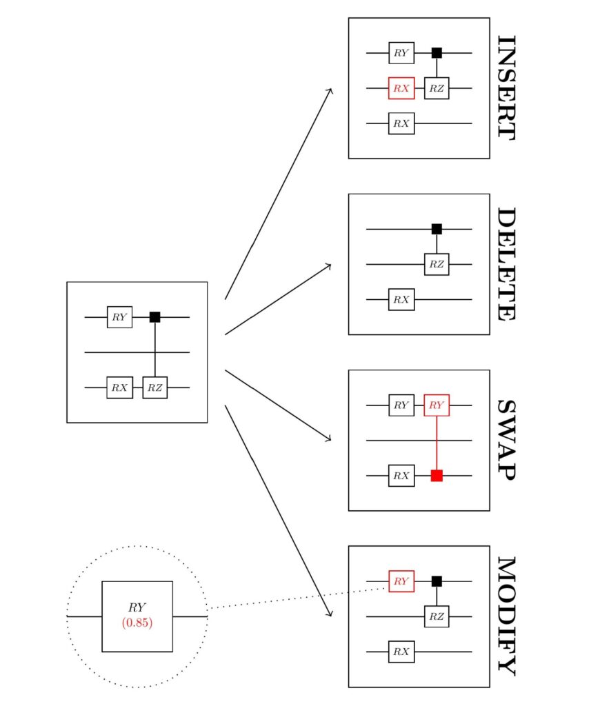
If the gates and their positions in a quantum circuit are fixed, the real-valued gate parameters can be optimized using a gradient method. However, this is not possible for the gate structure itself, as the mere existence of a gate, or its type and position, cannot be derived numerically. The researchers therefore decided to use evolutionary algorithms. These offer great flexibility, as it is sufficient to specify the recombination and mutation operators to guarantee that the method will produce a good result. To mutate a quantum circuit, for example, gates are randomly added, removed, exchanged for other gates or the parameters are changed slightly. Through such small changes, the optimal circuit is gradually constructed over the generations.

Schematic representation of the mutation of an initial quantum circuit (left) and the resulting offspring (right). Offspring are created by inserting, deleting, exchanging or modifying gates.
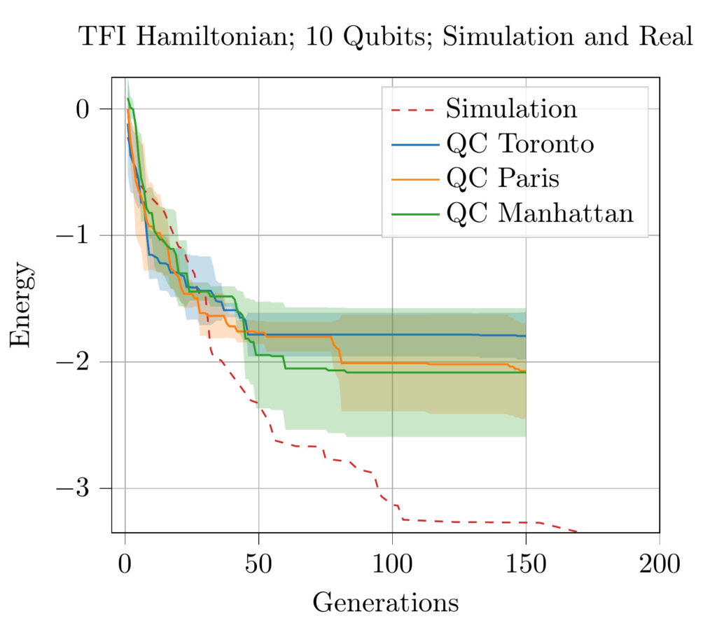
In their paper, the researchers were not only able to simulate this process, but also successfully carry it out on real quantum computers with up to 20 qubits. They thus showed that evolutionary optimization can be used effectively instead of the usual gradient methods for quantum computing problems. As a result, not only can parameters of fixed gate structures be learned, but also more compact quantum circuits can be found that require fewer gates.
The graph below shows the optimization process on various IBM quantum computers and in a simulation. In all cases, it can be observed that the energy decreases over the generations of the evolutionary algorithm, meaning that a good solution is gradually approximated.

Performance of the evolutionary algorithm on 10 qubits, executed on several quantum computers (colored lines) and simulated (dashed line).
Even more than half a century after its development, evolutionary optimization is still proving to be a flexible and powerful tool for cutting-edge applications. This is also the case in quantum computing, where gradient-based methods reach their limits.
Weitere Informationen im zugehörigen Paper:
Gradient-free quantum optimization on NISQ devices Lukas Franken, Bogdan Georgiev, Sascha Mücke, Moritz Wolter, Nico Piatkowski, Christian Bauckhage. Arxiv, 2020, PDF.
