With the advancement of digitalization in our society, the volume of collected data has become enormously large. This is especially relevant for Machine Learning, as large datasets generally lead to more meaningful results (read more about dataset size requirements in Machine Learning in the blog post How much data does Artificial Intelligence need?). However, this significantly impacts the computational time and memory complexity required for training a learning algorithm—and in many cases, these requirements (e.g., in real-time applications) cannot be met. Here, principal component analysis can help solve the problem. Below, you’ll learn how this tool works for dimensionality reduction of large, high-dimensional datasets.
What is dimensionality reduction?
Instead of reducing the number of data points that the algorithm learns from—which could negatively affect the quality of the trained model—we use a different approach. It is equally possible to reduce the number of features in the given data. The number of features is also referred to as the data’s dimensionality.
There are two main methods to reduce the dimensionality of a dataset, used both in data analysis and preprocessing for Machine Learning algorithms:
- Feature Selection: This involves selecting only a subset of the available features and then describing the data solely by the selected features.
- Feature Projection: Here, each data point is projected to a point with fewer features.
An important point here is that the features of the reduced point do not correspond to the original features—the reduced point as a whole just needs to resemble its counterpart from the original dataset.
Dimensionality reduction by projection
To better understand principal component analysis (PCA) and the concept of feature projection in general, it’s helpful to understand the (mathematical) concept of projection more deeply. So, what is projection? A projection is a function that changes an input point so that it can be described with fewer components. This can be understood as a type of shadow casting: the shadow of an originally three-dimensional point can be represented either as another three-dimensional point in the same space—depending on the light source and the surface onto which the shadow is cast. Alternatively, it can also be represented as a two-dimensional point on the plane where the shadow is cast.
To illustrate this with an example, let’s look at a regular cube being illuminated by a light source, casting its shadow on the ground on which it sits.

Figure 1: Sketch of a cube shadow
If we view the cube as a collection of points in three-dimensional space, its shadow is the set of points that results when the original points are projected onto the two-dimensional plane defined by the ground. This projection plane is defined by the projection function and doesn’t necessarily have to be two-dimensional. Therefore, the surface onto which the projection is made is generally called a subspace, and its dimensionality determines the reduced dimension of the data points. Furthermore, the shadow casting (onto the same two-dimensional plane) can be changed by moving the light source to another position. If we center the light source above the cube so that the cube is directly between the ground and the light source, the shadow appears directly beneath the cube. Since in this projection, the line connecting an original cube point to its corresponding shadow point is precisely orthogonal (i.e., at a 90-degree angle) to the ground, or the projection surface, we refer to this as an orthogonal projection.
Since such orthogonal projections minimize the distance between an original point and its corresponding shadow point (by the Pythagorean theorem), thereby preserving as much information from the original point as possible, the following method for reduction is restricted exclusively to finding the best possible orthogonal projection.
Principal component analysis
An example of dimensionality reduction by projection is Principal Component Analysis (PCA). PCA projects a set of data points onto a subspace, where the subspace is chosen so that the variance of the orthogonally projected data points is maximized. By maximizing the spread of the reduced data points, it is possible, in the case of classified data, to achieve good separability of the different classes (Classification in Machine Learning). The dimension $k$ of the subspace is specified by the user of PCA and determines how many coordinate axes the subspace is described by. These $k$ coordinate axes are also known as principal components.
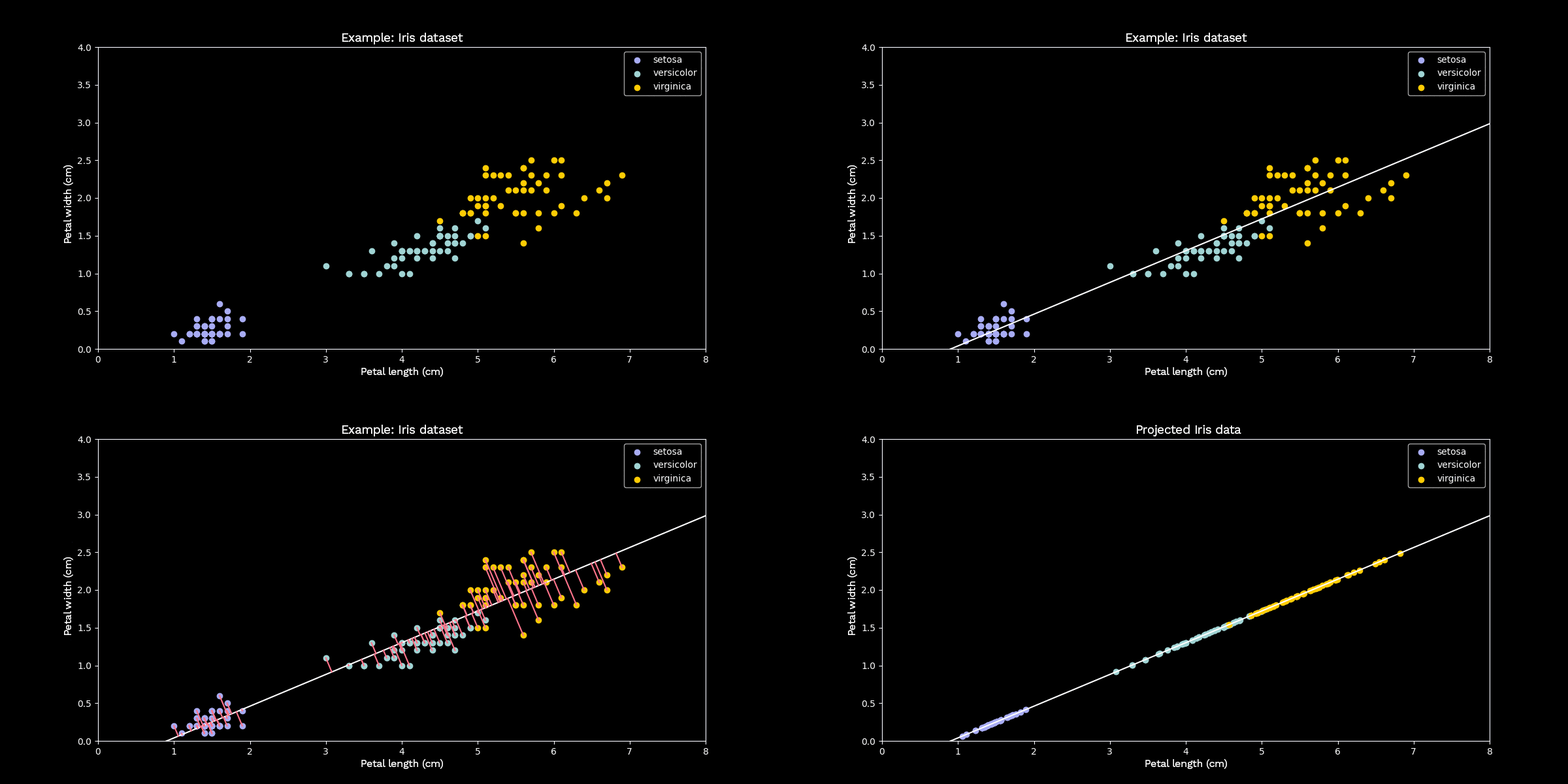
If a visual inspection of the data is possible, meaning that the original data has a maximum dimension of three, the first principal component can be seen as the direction of the greatest spread of the data. Each successive principal component points in the direction of the next greatest spread of the data, with the additional constraint that it is orthogonal to all previous principal components. To demonstrate this process with an example, we use Fisher’s Iris dataset—a dataset familiar to data scientists—which describes three different species of iris flowers with 150 examples and four features each. In the following example, we limit ourselves to two features for visualization purposes. These two features are the petal width and petal length measurements of each recorded plant.

Figure 2: Principal component analysis using the Iris dataset as an example
Now we apply PCA to this example to reduce the data to dimension $k = 1$. To do this, we look for the line through the data that maximizes the variance of the (orthogonally) projected data points. This line represents the one-dimensional subspace onto which PCA projects the data points. The above example shows that even after dimensionality reduction, the classes are still fairly distinguishable.
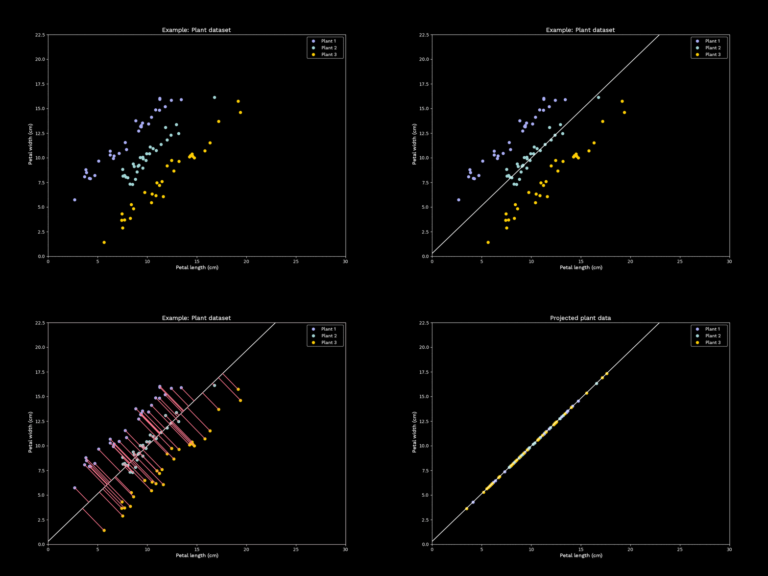
However, this is not always the case. Furthermore, applying PCA to classified data can lead to previously distinguishable classes becoming completely overlapping after dimensionality reduction, so that clear differences between the classes can no longer be detected. To illustrate this, we again examine a set of two-dimensional data points with fictitious measurements for three different plant types:

Figure 3: Principal component analysis with unfavorable sample data
The last example shows that Principal Component Analysis, especially as an intermediate step in a classification problem, should be applied cautiously.
Conclusion
Dimensionality reduction is an important area of Machine Learning. In addition to reducing computational time and memory requirements, it can also help counteract unwanted noise. Essentially, dimensionality reduction is nothing other than reducing the number of features in a given dataset. It fundamentally involves distinguishing between the methods of feature selection and feature projection. Principal Component Analysis is an example of the latter, which projects data onto the subspace that contains the most variance.
Next week, we’ll continue discussing dimensionality reduction for large datasets. We’ll present another method and outline its advantages and disadvantages.
