“Like!”. Every day, we receive personalized recommendations for products or content—whether shopping on various online marketplaces, streaming movies and music, or using social media platforms. These recommendations are powered by recommendation systems that rely on Machine Learning methods. In the field of recommendation systems, Graph Neural Networks (GNNs) are increasingly being applied. These types of artificial neural networks work with graph-structured data, making them ideal for analyzing user-product interactions encoded as graphs, enabling predictions about user behavior. The resulting graphs often consist of billions of nodes and edges and evolve dynamically, as new users sign up daily and additional products are constantly added. GraphSAGE extends the idea of classical Convolutional Neural Networks to graphs by introducing a sampling strategy and aggregation functions, enabling the learning of node features in extremely large and dynamically growing graphs. A well-known example of GraphSAGE’s use is Pinterest’s recommendation system, which employs the algorithm to create personalized suggestions for users. Similarly, UberEats uses a modified version of GraphSAGE to suggest suitable food options to consumers. In this blog post, we take a closer look at the GraphSAGE algorithm. For an introduction to Graph Neural Networks, we recommend the blog post “Graph Neural Networks: An introduction to the world of graph-based AI models.”

Selecting neighbors: “neighborhood sampling”
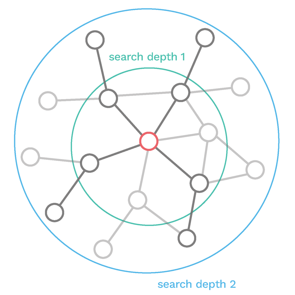
Training a GNN model on a large graph often presents two practical challenges that can impact the model’s accuracy and efficiency. First, processing graphs with billions of nodes is computationally expensive and requires significant storage space. Second, the neighborhood size of nodes can vary greatly, with some nodes having an exceptionally high number of neighbors. These high-degree nodes can heavily influence the model, as they receive information from many neighbors. This leads to enormous computational effort and can distort the representation of other nodes, ultimately affecting the model’s accuracy. To address these issues, a fixed number of neighbors is selected for each node for message exchange. This neighborhood sampling process involves the following steps:
- Define the search depth $k$: Perform $k$ iterations of message passing.
- Select neighbors at each search depth: Selection can be uniformly random (sampling with replacement) or based on a method suitable for the application.
These steps are repeated for each node, ultimately resulting in a subgraph with all nodes needed for further computations.

Information processing: aggregation functions
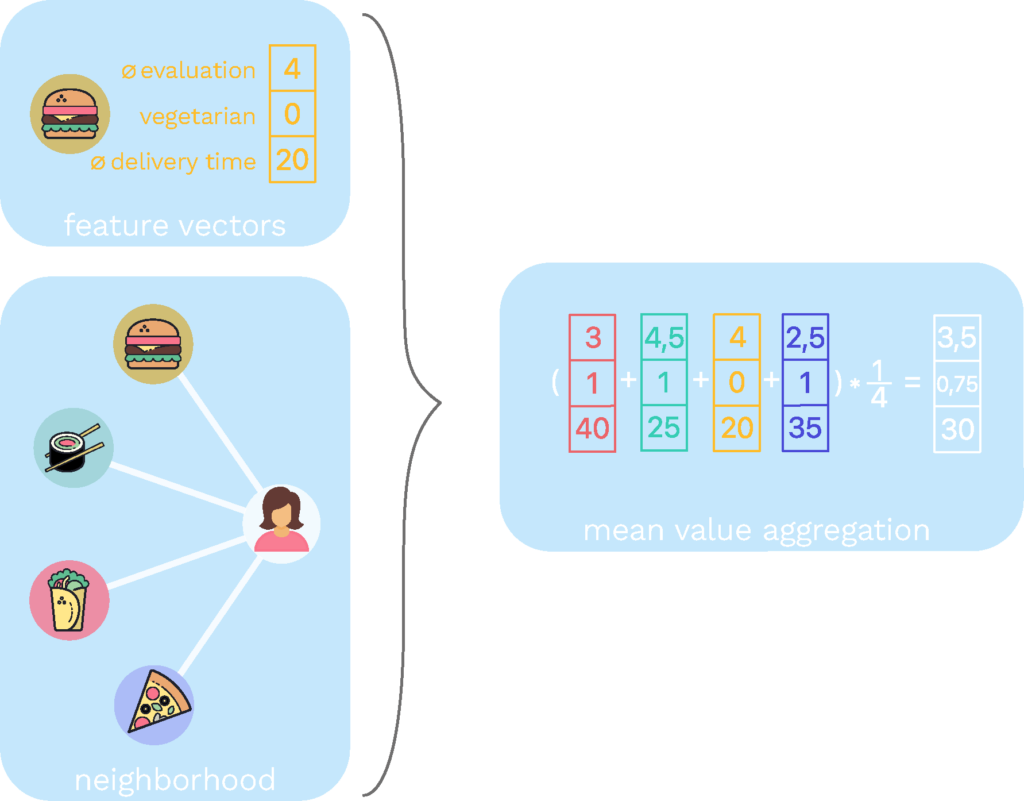
The aggregation function describes how the information of the neighborhood described above is merged and processed to derive information about the target node. In order to improve the aggregation functions and thus the predictions of the model, each aggregation function has a weight matrix as a parameter that determines the weighting of the neighboring nodes. The weightings, and thus the relevance of individual neighboring nodes, are adjusted by training the model using methods such as gradient descent. The choice of aggregation function depends on the specific task and can significantly influence the performance of the algorithm. Some examples of aggregation functions are the mean function, which calculates the average of the features in the neighborhood, or the maximum function, which filters out the most representative feature.
How does GraphSAGE learn?
With the basics established, we can now examine the complete GraphSAGE learning algorithm. It takes a graph as input and outputs a vector representation for each node. The following steps are applied:
- Initialization: The initial features of the nodes are used for their initial representation.
- Neighborhood Sampling: The neighborhood is sampled as described above.
- Aggregation: An aggregation function generates a representation of each node’s neighborhood.
- Concatenation: The aggregated features of the neighbors are concatenated with the current node’s representation to contribute to an improved overall representation.
- Fully Connected Layer with Activation Function: The fully connected layer consists of a weight matrix adjusted during training to achieve the optimal combination of features. The activation function captures non-linear relationships between nodes.
- Normalization: To standardize the scaling of node representations and improve model stability, the new feature vectors of the nodes are normalized by dividing each vector by its Euclidean norm.
- Optimization of Model Parameters: Gradient descent is used to optimize the model parameters.
Steps 2–7 are repeated to iteratively improve the aggregation functions and node representations.
The final representations of the nodes can be used as input for Machine Learning models to perform various tasks, such as classification or relationship prediction. By leveraging these node representations, models can utilize the knowledge about the graph’s structure and relationships more effectively, leading to better predictions.
Conclusion
GraphSAGE is a powerful Machine Learning method for analyzing graph-structured data. It is used in recommendation systems to predict user behavior based on interactions with products or content. The GraphSAGE method extends the idea of the message-passing model by incorporating a sampling strategy and aggregation functions, allowing for the learning of node features in extremely large and dynamically growing graphs. GraphSAGE is a promising approach for processing large graph data and has applications beyond recommendation systems, including social network analysis, molecular biology, and fraud detection.
Even though the semester is still in full swing, our ML Classroom series is taking a break for the semester holidays. We’ll be back next month with exciting contributions from our Lamarr researchers and insights into real-world applications. So, stay tuned! Don’t want to miss a post? Sign up for our newsletter and follow us on X and LinkedIn.
