When it comes to making Artificial Intelligence explainable, the focus is often on identifying the reason behind a model’s decision (see our blog post, “Why AI needs to be explainable”). Let’s take a step back to the creation of such a model: the so-called model training. To understand how a model was created, the metadata of the training process should be recorded. This is referred to as experiment tracking. Metadata for a training process can include various parameters, hyperparameters, and metrics. With sufficient information, repeating the training process can yield the same or at least a comparable result. This is also essential for evaluating models created through different training processes. Differences in results can then be better attributed to the variations in data or metadata. A clear overview of the model’s results allows for selecting the best model.
During the exploratory phase of the ML engineering process, model training and achieving good metrics often take center stage, while documenting the results tends to be neglected. Good documentation, however, is especially crucial in lengthy and complex processes. It helps maintain oversight and ultimately achieve a reproducible result.
Currently, experiments are often documented as text files, and different versions are frequently marked by suffixes in file names such as “Model_v1, Model_v2, Model_v2_approach1”. Automating the recording of training processes and versioning work states can ease the workflow and lead to clear documentation. A tool that can assist in these steps is MLflow, which we will introduce with a sample workflow in this article.
The illustrative sample workflow can be followed using code examples on your own computer. A Linux environment is recommended, and Git and Anaconda should already be installed.
A Sample Workflow in MLflow
The goal of this sample workflow is to develop a model that classifies wine into quality levels using the Wine Quality dataset. This is a classification problem (see “What are the types of Machine Learning?” for more information on classification). Wines are assigned a quality score (output variable) between 0 and 10 based on input variables such as fixed acidity, volatile acidity, citric acid, residual sugar, chlorides, free sulfur dioxide, total sulfur dioxide, density, pH, sulfates, and alcohol content. We use code from the official MLflow repository as the foundation.
Step 1: Setting Up Code and MLflow
First, we need to set up the code and MLflow. We obtain the code by accessing MLflow’s central code repository. This so-called repository can be cloned using Git via any command line interface. However, before doing so, we should navigate to the directory where we want to store the code. After cloning, we move into the directory “./mlflow/examples/sklearn_elasticnet_wine/”. This directory already contains a notebook file train.ipynb and a conda.yaml file, which allows us to create a predefined Anaconda environment called tutorial. We do this using the command: conda env create -f conda.yaml
To use the created Conda environment within a Jupyter Notebook, we first need to install the IPython kernel in our environment. Then, we register the current environment under a name (e.g., also tutorial), making it accessible within Jupyter Notebook. If not already installed, jupyterlab can be added to launch Jupyter Notebooks.
Finally, we start our Jupyter Notebook with the command: jupyter notebook
# Navigate to any directory where the repository should be cloned
cd /home/username/repository

# Set up Conda and Jupyter Notebook
git clone https://github.com/mlflow/mlflow.git
cd mlflow/examples/sklearn_elasticnet_wine
conda env create -f conda.yaml
conda activate tutorial

# Use the Conda environment in Jupyter Notebook
conda install -c anaconda ipykernel
ipython kernel install --user --name=tutorial
conda install -c conda-forge jupyterlab

# Start Jupyter Notebook
jupyter notebook
The Jupyter notebook is now running in the current command window, in which a URL is also provided via which the user interface of the Jupyter notebook can be called up in the browser.
In a new command window, we now move to the sklearn_elasticnet_wine folder again. To ensure that the information we want is tracked, we should activate the tutorial environment, as MLflow is already installed in it. We can then call up the MLflow user interface from the sklearn_elasticnet_wine folder using the mlflow ui command. This starts the so-called tracking server, which is then accessible via http://localhost:5000 by default. MLflow stores the information on the tracked training processes in the mlruns folder. These are loaded by MLflow and displayed on the tracking server.
# Start the mlflow tracking server
cd mlflow/examples/sklearn_elasticnet_wine
conda activate tutorial
mlflow ui
The commands listed often do not work without problems under Windows. The following points may help with the execution:
- Set the path to the Anaconda installation if Anaconda was assumed to be installed in the C:tools folder: set PATH=%PATH%;C:\tools\Anaconda3;C:\tools\Anaconda3\Scripts\
- Activate the Conda environment “tutorial” without an explicit “conda” call: activate tutorial
- Copy the following files from C:\tools\Anaconda3\Library\bin to C:\tools\Anaconda3\DLLs:
- libcrypto-1_1-x64.*
- libssl-1_1-x64.*
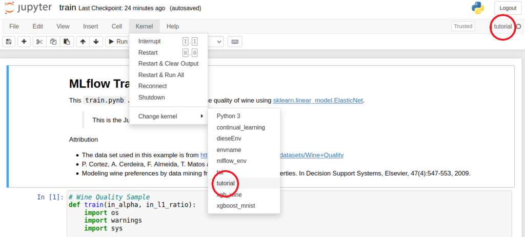
Jupyter Notebook “train” with activated “tutorial” kernel
Step 2: Preparing a Jupyter Notebook for MLflow
In order to be able to use the notebook without restrictions, our Conda environment must be activated in the notebook. We have already enabled this in the first code block. Now we can open the user interface of the Jupyter notebook with the URL provided in step 1 and select our “tutorial” kernel via “Kernel” à “Change kernel” and prepare the notebook for tracking. We need to define the information to be tracked in the notebook. If we look at the train.ipynb notebook, we can see that we first call the mlflow.start_run() function. This starts a run for which the subsequent indented code is executed. In our case, the run includes a training process. If an error occurs or after the indented code has been executed, the run is automatically terminated. The indented code calls the functions mlflow.log_param() and mlflow.log_metric() to log parameters and metrics, and finally mlflow.sklearn.log_model() to save the specific sklearn model.
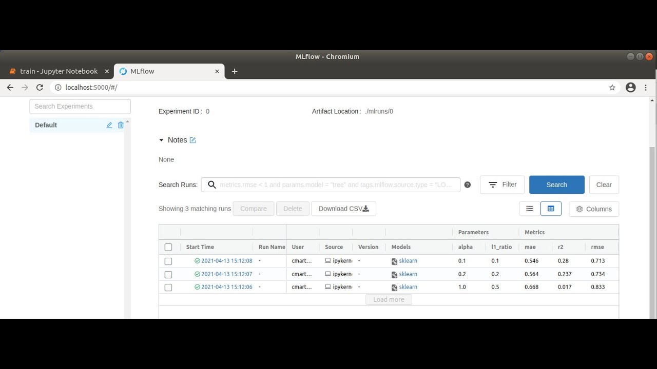
In the following cells of the notebook, three training procedures are defined with different values for the parameters alpha (amount of penalty for including irrelevant features) and l1_ratio (weighting between the two standard regularization methods L1 and L2). If we run the entire notebook, these training procedures are stored as runs in MLflow, which we can view in the MLflow user interface.
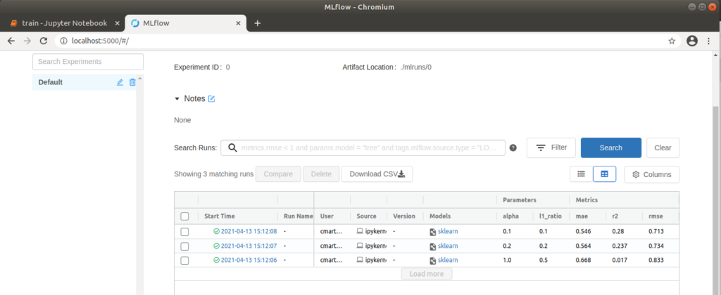
MLflow user interface with three executed runs
Step 3: Viewing Results in the MLflow Interface
We can now open http://localhost:5000 in our browser and select the “Default” project in the MLflow interface to compare the executed runs. To do this, we first wait until a green tick appears on all runs to indicate that the processes have been completed. We then select all three runs and click on “Compare”. In the window that opens, parameters that differ in the three runs are highlighted in color. In our case, these are the two parameters alpha and l1_ratio. We can also compare the runs visually using various plots. For example, if we click on “rmse” (root of the mean squared error), a graph is displayed which clearly shows that the “rmse” for run 1 is the lowest. This means that the difference between observed and predicted data is the smallest and therefore the model is best adapted to the data used. Further settings can be made on the left-hand side; for example, “r2” (coefficient of determination), also for assessing the fit of the model to the data, and “mae” (mean absolute error) for assessing the accuracy of the model’s predictions, can also be displayed. Depending on the application, it is advisable to try out different display options.
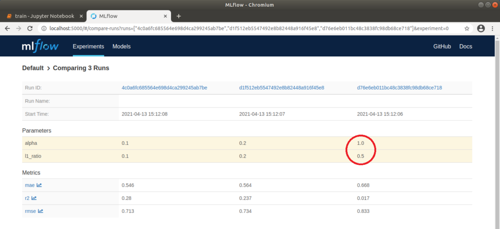
MLflow: Tabular comparison of the parameters and metrics of three runs
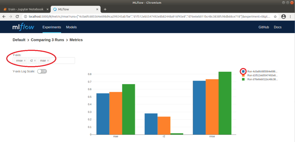
MLflow: Graphical comparison of the metrics of three runs
Step 4: Examining the Best Run in Detail
Run 1 with the values alpha=0.1 and l1_ratio=0.1 delivered the best result with an “rmse” of approx. 0.71. We can explicitly call up meta information on this run via the run ID. If we click on the graphic above, a pop-up also opens, which we can use to jump directly to a run. Here we can add notes and view the exact parameters and metrics again. We can also view the corresponding model files under “Artifacts”. A conda.yaml can also be supplied, under which the model can be loaded or trained on other computers. This is generated automatically without an explicit definition. Clicking on the “model” folder also displays a Python code example that can be used to make a prediction.
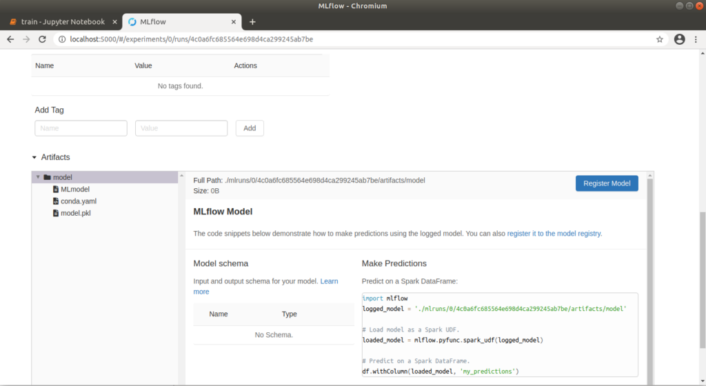
Model artifact retrievable in MLflow
Step 5: Using the Model for Predictions
To obtain the model we have created and thus make a prediction, we can use MLflow’s code suggestion as a guide. We adapt this by retrieving the appropriate run_id from the URL (http://localhost:5000/#/experiments/experiment_nummer/runs/run_id) and inserting it into the code. We write the code in a new cell in our notebook. We create the input data for the model manually in the code as input_data:
import mlflow
logged_model = './mlruns/0/run_id/artifacts/model' # insert run_id here
# Load model as a PyFuncModel.
loaded_model = mlflow.pyfunc.load_model(logged_model)
# Predict on a Pandas DataFrame.
import pandas as pd
input_data = {'fixed acidity': [8.5], 'volatile acidity': [0.26], 'citric acid': [0.21], 'residual sugar': [16.2], 'chlorides': [74], 'free sulfur dioxide': [41], 'total sulfur dioxide': [197], 'density': [998], 'pH': [3.02], 'sulphates': [0.5], 'alcohol': [9.8]}
prediction = loaded_model.predict(pd.DataFrame(input_data))
print("prediction = "+str(prediction[0]))
After running the cell, we receive the rating for the wine we have defined. If we play around a little, we quickly notice that the model’s rating is influenced by a very high or low alcohol content alone. 🙂
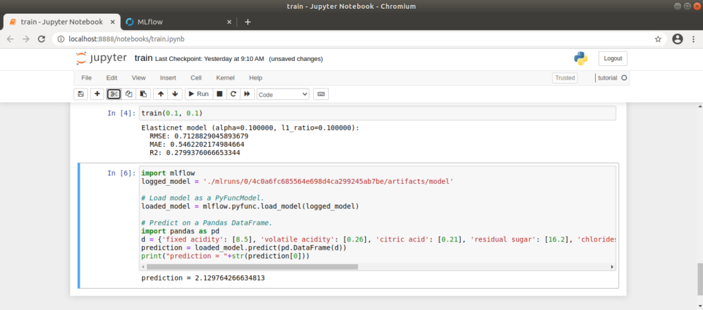
For the manually created input data, the model obtained here provides a value of approx. 2.1
Tracking, Tracking, Tracking, …
Our experiments can be automatically tracked by MLflow with just a few additional lines of code. This gives us a better overview of which metrics we achieve with which parameters, and we can assign our developed models to a specific training process, to which we can in turn assign a specific training environment.
Finally, it should be mentioned that the static Wine-Quality dataset was used here. However, just as models and parameters can change in the real world, it is also possible to change the source code and the underlying data. In the next blog entries in this series, I will therefore look at how source code and data can be managed during exploration.
More information about the implementation in the corresponding video:
