Decision Trees are a highly popular tool in Machine Learning (ML). They represent a hierarchical, tree-like structure that graphically illustrates the decision-making process. They can assist in making decisions or in effectively explaining and visualizing one’s decisions to others. However, as the amount of data we use for decision-making grows, the decision-making process becomes more complex. Pruning can be used to trim decision trees and keep them manageable.
What are Decision Trees used for?
Decision Trees can be employed in various domains. Their general task is to classify a set of data objects or to represent rules based on existing knowledge. Examples of applications include classifying bank customers based on their creditability, using attributes for decision-making such as homeownership or marital status. Another example is providing relevant product recommendations for online shop customers based on their previous interests and purchases. In the field of medicine, decision trees could also be used to classify tumors as benign or malignant, using attributes like tumor size or texture.
How are Decision Trees structured?
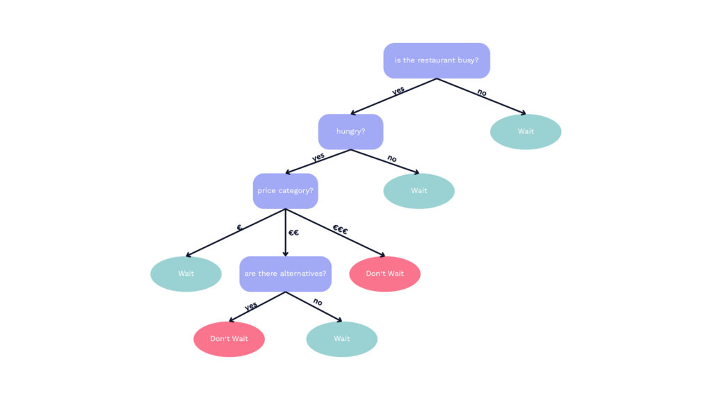
The tree starts with an initial root node, from which various paths lead to leaf nodes through different decision levels, representing the ultimate decisions. Each preceding intermediate step, depicted by the respective inner node, signifies a decision rule based on an attribute. This decision rule can be either a binary yes-no decision or a multi-layered decision, for instance, for each attribute value. This is illustrated in the following example. In this scenario, you face the decision of whether to wait for a free table in a crowded restaurant. For decision-making, the tree considers attributes such as the price of the food, your level of hunger, and the restaurant’s occupancy. The first attribute involves a decision between multiple attribute values (three price tiers). If you follow the relevant decision edges to a leaf node, it will indicate whether it’s more reasonable to wait or not to wait.

The selection of attributes for each decision node is done by maximizing information gain. This is calculated using entropy and the remaining information need after attribute selection. The attribute chosen for the decision node is the one that achieves the highest information gain, thus maximizing it.
What are the pros and cons of using Decision Trees?
As we have seen, decision trees are applicable in many areas and are very intuitive and easy to follow in their structure. Therefore, they are suitable for work and collaboration with partners who are inexperienced in the field of Machine Learning. Additionally, they work for both categorical and numerical data types, with the type of decision node potentially needing adjustment. Another advantage is their combinability with an ensemble learning method, where we use multiple decision trees. Here the final decision is often determined by a majority vote of individual results. An example of this are Random Forests, which use multiple different, uncorrelated decision trees for classification following the Bagging principle. Furthermore, using Decision Trees requires less data cleaning, meaning the data does not need extensive preprocessing compared to other data modelling techniques. However, the tree can still be influenced by noise under certain circumstances, especially if it is overly fitted to the training dataset, which is known as overfitting. Additionally, the use of Decision Trees can become problematic with overly complex datasets, where the tree can quickly become large and difficult to interpret. In such cases, it goes against the usual advantage of the structure being easily understandable.
Decision Tree Pruning
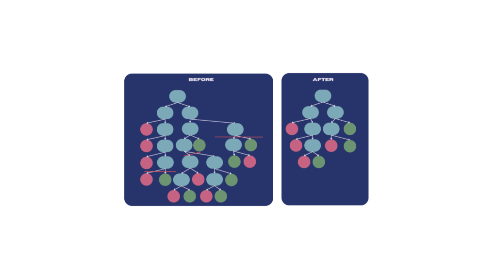
With the advent of Big Data, it is getting more common for Decision Trees to become too large and less interpretable. To counteract this issue and prevent Decision Trees from becoming overly large and complex, it is advisable to use only the most critical decisions. This involves excluding unimportant and redundant differentiations to keep the tree smaller and more manageable. This process is known as Pruning.
It is important to note that we only prune branches that are no longer relevant and do not worsen the result, but ideally, improve it. Typically, only those branches are pruned that satisfy specific criteria. Depending on the algorithm, these criteria indicate whether a particular branch is irrelevant and degrades the performance or does not enhance it. By using different algorithms, you can adapt the criteria and the pruning process to fit the specific example.

Pruning Techniques
Now, the previously mentioned general differences in pruning algorithms will be explained in more detail.
There are two ways to prune a decision tree. On the one hand, you can consider an already completed decision tree and subsequently cut off branches that are no longer needed. This is known as Post-Pruning. The other option is called Pre-Pruning, where redundant or less important branches are omitted during the creation of the decision tree.
Post-Pruning is more commonly used and replaces subtrees with nodes when they are deemed unnecessary. Since there was already a completed decision tree at the outset, after pruning, we can see the improvements in accuracy and complexity in the pruned tree and compare it with the original tree.
Pre-Pruning uses a stopping criterion, preventing the tree from further expansion. An example of such a stopping criterion is the depth of the tree, meaning it is predetermined how many consecutive decision nodes are allowed. This process is generally considered efficient because it keeps the tree small from the beginning and does not require the entire dataset. However, it can lead to premature pruning without considering all the information, resulting in the loss of important information. This effect is referred to as the Horizon Effect.
The direction in which the tree is traversed during Post-Pruning is called Bottom-Up or Top-Down Pruning. As their names imply, this describes the respective traversal direction of the algorithm, from the root to the leaves or vice versa.
Bottom-Up starts at the lowest point and then recursively moves upward, while Top-Down Pruning begins at the root and moves downward to the leaves. For Top-Down Pruning, there is a risk that subtrees may be pruned prematurely, even if relevant nodes are still below.
Conclusion
Decision trees are a practical tool for visually representing decision processes for classification or rule presentation. However, in today’s era of ever-increasing volumes of data, problems can arise as the tree becomes too complex or difficult to understand. Pruning can help address this issue by removing branches in the tree that are not needed for decision-making and are therefore redundant.
Would you like to delve deeper into the topic of pruning? In our next blog post, we will focus on the topic of pruning algorithms, in which we compare the two algorithms pessimistic error pruning and minimum error pruning.

